--- title: "Anemia prevalence: an `rdhs` example" author: "OJ Watson, Jeff Eaton" date: "2018-09-24" output: rmarkdown::html_vignette: keep_md: TRUE vignette: > %\VignetteIndexEntry{Anemia prevalence among women: an `rdhs` example} %\VignetteEngine{knitr::rmarkdown} %\VignetteEncoding{UTF-8} --- Anemia is a common cause of fatigue, and women of childbearing age are at particularly high risk for anemia. The package `rdhs` can be used to compare estimates of the prevalence of any anemia among women from Demographic and Health Surveys (DHS) conducted in Armenia, Cambodia, and Lesotho. # Setup Load the `rdhs` package and other useful packages for analysing data. ```r ## devtools::install_github("ropensci/rdhs") library(rdhs) library(data.table) library(ggplot2) library(survey) library(haven) ``` # Using calculated indicators from STATcompiler Anemia prevalence among women is reported as a core indicator through the DHS STATcompiler (https://www.statcompiler.com/). These indicators can be accessed directly from R via the DHS API with the function `dhs_data()`. Query the API for a list of all StatCompiler indicators, and then search the indicators for those that have `"anemia"` in the indicator name. API calls return `data.frame` objects, so if you prefer to use `data.table` objects then convert afterwards, or we can set this up within our config using `set_rdhs_config`. ```r library(rdhs) set_rdhs_config(data_frame = "data.table::as.data.table") indicators <- dhs_indicators() tail(indicators[grepl("anemia", Label), .(IndicatorId, ShortName, Label)]) ``` ``` ## IndicatorId ShortName Label ## 1: CN_ANMC_C_SEV Severe anemia (<7.0 g/dl) Children with severe anemia ## 2: AN_ANEM_W_ANY Any Women with any anemia ## 3: AN_ANEM_W_MLD Mild Women with mild anemia ## 4: AN_ANEM_W_MOD Moderate Women with moderate anemia ## 5: AN_ANEM_W_SEV Severe Women with severe anemia ## 6: AN_ANEM_M_ANY Any anemia Men with any anemia ``` The indicator ID `"AN_ANEM_W_ANY"` reports the percentage of women with any anemia. The function `dhs_data()` will query the indicator dataset for the value of this indicator for our three countries of interest. First, use `dhs_countries()` to query the list of DHS countries to identify the DHS country code for each country. 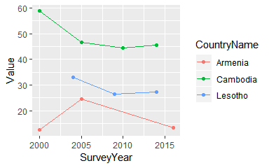```r countries <- dhs_countries() dhscc <- countries[CountryName %in% c("Armenia", "Cambodia", "Lesotho"), DHS_CountryCode] dhscc ``` ``` ## [1] "AM" "KH" "LS" ``` Now query the indicators dataset for the women with any anemia indicator for these three countries. ```r statcomp <- dhs_data(indicatorIds = "AN_ANEM_W_ANY", countryIds = dhscc) statcomp[,.(Indicator, CountryName, SurveyYear, Value, DenominatorWeighted)] ``` ``` ## Indicator CountryName SurveyYear Value DenominatorWeighted ## 1: Women with any anemia Armenia 2000 12.4 6137 ## 2: Women with any anemia Armenia 2005 24.6 6080 ## 3: Women with any anemia Armenia 2016 13.4 5769 ## 4: Women with any anemia Cambodia 2000 58.8 3634 ## 5: Women with any anemia Cambodia 2005 46.7 8219 ## 6: Women with any anemia Cambodia 2010 44.4 9229 ## 7: Women with any anemia Cambodia 2014 45.4 11286 ## 8: Women with any anemia Lesotho 2004 32.9 3008 ## 9: Women with any anemia Lesotho 2009 26.3 3839 ## 10: Women with any anemia Lesotho 2014 27.3 3297 ``` ```r ggplot(statcomp, aes(SurveyYear, Value, col=CountryName)) + geom_point() + geom_line() ```

# Analyse DHS microdata ## Identify surveys that include anemia testing The DHS API provides the facility to filter surveys according to particular characteristics. We first query the list of survey characteristics and identify the `SurveyCharacteristicID` that indicates the survey included anemia testing. The first command below queries the API for the full list of survey characteristics, and the second uses `grepl()` to search `SurveyCharacteristicName`s that include the word 'anemia'. ```r surveychar <- dhs_survey_characteristics() surveychar[grepl("anemia", SurveyCharacteristicName, ignore.case=TRUE)] ``` ``` ## SurveyCharacteristicID SurveyCharacteristicName ## 1: 15 Anemia questions ## 2: 41 Anemia testing ``` The `SurveyCharacteristicID = 41` indicates that the survey included anemia testing. Next we query the API to identify the surveys that have this characteristic and were conducted in our countries of interest. ```r surveys <- dhs_surveys(surveyCharacteristicIds = 41, countryIds = dhscc) surveys[,.(SurveyId, CountryName, SurveyYear, NumberOfWomen, SurveyNum, FieldworkEnd)] ``` ``` ## SurveyId CountryName SurveyYear NumberOfWomen SurveyNum FieldworkEnd ## 1: AM2000DHS Armenia 2000 6430 203 2000-12-01 ## 2: AM2005DHS Armenia 2005 6566 262 2005-12-01 ## 3: AM2016DHS Armenia 2016 6116 492 2016-04-01 ## 4: KH2000DHS Cambodia 2000 15351 140 2000-07-01 ## 5: KH2005DHS Cambodia 2005 16823 257 2006-03-01 ## 6: KH2010DHS Cambodia 2010 18754 310 2011-01-01 ## 7: KH2014DHS Cambodia 2014 17578 464 2014-12-01 ## 8: LS2004DHS Lesotho 2004 7095 256 2005-01-01 ## 9: LS2009DHS Lesotho 2009 7624 317 2010-01-01 ## 10: LS2014DHS Lesotho 2014 6621 462 2014-12-01 ``` Finally, query the API identify the individual recode (IR) survey datasets for each of these surveys ```r datasets <- dhs_datasets(surveyIds = surveys$SurveyId, fileType = "IR", fileFormat="flat") datasets[, .(SurveyId, SurveyNum, FileDateLastModified, FileName)] ``` ``` ## SurveyId SurveyNum FileDateLastModified FileName ## 1: AM2000DHS 203 October, 05 2006 14:22:40 AMIR42FL.ZIP ## 2: AM2005DHS 262 February, 02 2010 10:38:12 AMIR54FL.zip ## 3: AM2016DHS 492 September, 21 2017 16:10:15 AMIR71FL.ZIP ## 4: KH2000DHS 140 October, 08 2007 12:31:53 KHIR42FL.zip ## 5: KH2005DHS 257 October, 18 2011 13:53:19 KHIR51FL.zip ## 6: KH2010DHS 310 October, 26 2011 11:11:07 KHIR61FL.ZIP ## 7: KH2014DHS 464 July, 28 2017 10:58:10 KHIR73FL.ZIP ## 8: LS2004DHS 256 July, 31 2007 13:14:31 LSIR41FL.ZIP ## 9: LS2009DHS 317 November, 10 2015 10:51:05 LSIR61FL.ZIP ## 10: LS2014DHS 462 June, 14 2016 11:35:19 LSIR71FL.ZIP ``` ## Download datasets To download datasets we need to first log in to our DHS account, by providing our credentials and setting up our configuration using `set_rdhs_config()`. This will require providing as arguments your `email` and `project` for which you want to download datasets from. You will then be prompted for your password. You can also specify a directory for datasets and API calls to be cached to using `cache_path`. In order to comply with CRAN, this function will also ask you for your permission to write to files outside your temporary directory, and you must type out the filename for the `config_path` - "rdhs.json". (See [introduction vignette](https://docs.ropensci.org/rdhs/articles/introduction.html) for specific format for config, or `?set_rdhs_config`). ```r ## set up your credentials set_rdhs_config(email = "jeffrey.eaton@imperial.ac.uk", project = "Joint estimation of HIV epidemic trends and adult mortality") ``` After this the function `get_datasets()` returns a list of file paths where the desired datasets are saved in the cache. The first time a dataset is accessed, `rdhs` will download the dataset from the DHS program website using the supplied credentials. Subsequently, datasets will be simply be located in the cached repository. ```r datasets$path <- unlist(get_datasets(datasets$FileName)) ``` ``` ## Logging into DHS website... ``` ``` ## Creating Download url list from DHS website... ``` ## Identify survey variables Anemia is defined as having a hemoglobin (Hb) <12.0 g/dL for non-pregnant women or Hb <11.0 g/dL for currently pregnant women^[https://www.measureevaluation.org/prh/rh_indicators/womens-health/womens-nutrition/percent-of-women-of-reproductive-age-with-anemia]. To calculate anemia prevalence from DHS microdata, we must identify the DHS recode survey variables for hemoglobin measurement and pregnancy status. This could be done by consulting the DHS recode manual or the .MAP files accompanying survey datasets. It is convenient though to do this in R by loading the first individual recode dataset and searching the metadata for the variable names corresponding to the hemoglobin measurement and pregnancy status. ```r head(search_variable_labels(datasets$FileName[10], "hemoglobin")[,1:2]) ``` ``` ## variable ## 1 v042 ## 2 v452c ## 3 v453 ## 4 v455 ## 5 v456 ## 6 hw52_1 ## description ## 1 Household selected for hemoglobin ## 2 Read consent statement - hemoglobin ## 3 Hemoglobin level (g/dl - 1 decimal) ## 4 Result of measurement - hemoglobin ## 5 Hemoglobin level adjusted for altitude and smoking (g/dl - 1 decimal) ## 6 Read consent statement - hemoglobin ``` Variable `v042` records the household selection for hemoglobin testing. Variable `v455` reports the outcome of hemoglobin measurement and `v456` the result of altitude adjusted hemoglobin levels. ```r ir <- readRDS(datasets$path[10]) table(as_factor(ir$v042)) ``` ``` ## ## not selected selected ## 3203 3418 ``` ```r table(as_factor(ir$v455)) ``` ``` ## ## measured not present ## 3349 2 ## refused other ## 35 8 ## no measurement found in household missing ## 0 24 ``` ```r summary(ir$v456) ``` ``` ## Min. 1st Qu. Median Mean 3rd Qu. Max. NA's ## 24.0 118.0 130.0 145.6 141.0 999.0 3203 ``` Variable `v454` reports the current pregnancy status used for determining the anemia threshold. ```r search_variable_labels(datasets$FileName[1], "currently.*pregnant")[,1:2] ``` ``` ## variable description ## 1 v213 Currently pregnant ## 2 v454 Currently pregnant ``` ```r table(as_factor(ir$v454)) ``` ``` ## ## no/don't know yes missing ## 3276 142 0 ``` We also keep a number of other variables related to the survey design and potentially interesting covariates: country code and phase (`v000`), cluster number (`v001`), sample weight (`v005`), age (`v012`), region (`v024`), urban/rural residence (`v025`), and education level (`v106`). ```r vars <- c("SurveyId", "CountryName", "SurveyYear", "v000", "v001", "v005", "v012", "v024", "v025", "v106", "v042", "v454", "v455", "v456") ``` ## Extract survey data ```r datlst <- list() for(i in 1:nrow(datasets)){ if(file.exists(datasets$path[i])){ print(paste(i, datasets$SurveyId[i])) ir <- readRDS(datasets$path[i]) ir$SurveyId <- datasets$SurveyId[i] ir$CountryName <- datasets$CountryName[i] ir$SurveyYear <- datasets$SurveyYear[i] datlst[[datasets$SurveyId[i]]] <- ir[vars] } } ``` ``` ## [1] "1 AM2000DHS" ## [1] "2 AM2005DHS" ## [1] "3 AM2016DHS" ## [1] "4 KH2000DHS" ## [1] "5 KH2005DHS" ## [1] "6 KH2010DHS" ## [1] "7 KH2014DHS" ## [1] "8 LS2004DHS" ## [1] "9 LS2009DHS" ## [1] "10 LS2014DHS" ``` We use `rbind_labelled()` to combine datasets with labelled columns. The argument `labels` describes to combine variable levels for all datasets for `v024` (region) while providing a consistent set of value labels to be used for `v454` (currently pregnant) for all datasets. ```r dat <- rbind_labelled(datlst, labels = list(v024 = "concatenate", v454 = c("no/don't know" = 0L, "yes" = 1L, "missing" = 9L))) ``` ``` ## Warning in rbind_labelled(datlst, labels = list(v024 = "concatenate", v454 = c(`no/don't know` = 0L, : Some variables have non-matching value labels: v106, v455, v456. ## Inheriting labels from first data frame with labels. ``` ```r sapply(dat, is.labelled) ``` ``` ## SurveyId CountryName SurveyYear v000 v001 v005 ## FALSE FALSE FALSE FALSE FALSE FALSE ## v012 v024 v025 v106 v042 v454 ## FALSE TRUE TRUE TRUE TRUE TRUE ## v455 v456 DATASET ## TRUE TRUE FALSE ``` ```r dat$v456 <- zap_labels(dat$v456) dat <- as_factor(dat) ``` ## Data tabulations It is a good idea to check basic tabulations of the data, especially by survey to identify and nuances Exploratory analysis of variables ```r with(dat, table(SurveyId, v025, useNA="ifany")) ``` ``` ## v025 ## SurveyId urban rural ## AM2000DHS 3545 2885 ## AM2005DHS 4592 1974 ## AM2016DHS 3545 2571 ## KH2000DHS 2627 12724 ## KH2005DHS 4152 12671 ## KH2010DHS 6077 12677 ## KH2014DHS 5667 11911 ## LS2004DHS 1945 5150 ## LS2009DHS 1977 5647 ## LS2014DHS 2202 4419 ``` ```r with(dat, table(SurveyId, v106, useNA="ifany")) ``` ``` ## v106 ## SurveyId no education primary secondary higher missing ## AM2000DHS 5 24 5329 1072 0 ## AM2005DHS 7 24 5138 1397 0 ## AM2016DHS 5 406 2580 3125 0 ## KH2000DHS 4849 8182 2276 44 0 ## KH2005DHS 3772 9131 3771 149 0 ## KH2010DHS 3203 8796 6141 614 0 ## KH2014DHS 2233 7826 6535 984 0 ## LS2004DHS 169 4309 2520 97 0 ## LS2009DHS 114 3865 3277 368 0 ## LS2014DHS 81 2665 3354 521 0 ``` ```r with(dat, table(SurveyId, v454, useNA="ifany")) ``` ``` ## v454 ## SurveyId no/don't know yes missing ## AM2000DHS 6231 199 0 0 ## AM2005DHS 5967 158 441 0 ## AM2016DHS 5939 177 0 0 ## KH2000DHS 3312 296 62 11681 ## KH2005DHS 7685 501 212 8425 ## KH2010DHS 8906 475 0 9373 ## KH2014DHS 10883 663 0 6032 ## LS2004DHS 2857 203 0 4035 ## LS2009DHS 3740 173 103 3608 ## LS2014DHS 3276 142 0 3203 ``` ```r with(dat, table(SurveyId, v455, useNA="ifany")) ``` ``` ## v455 ## SurveyId measured not present refused other no measurement found in hh ## AM2000DHS 6137 5 264 24 0 ## AM2005DHS 6134 8 294 1 0 ## AM2016DHS 5807 11 295 0 0 ## KH2000DHS 3666 0 68 0 0 ## KH2005DHS 8182 2 185 5 0 ## KH2010DHS 9225 9 106 0 0 ## KH2014DHS 11390 8 13 2 0 ## LS2004DHS 3061 15 377 56 0 ## LS2009DHS 3896 1 78 5 0 ## LS2014DHS 3349 2 35 8 0 ## v455 ## SurveyId missing ## AM2000DHS 0 0 ## AM2005DHS 129 0 ## AM2016DHS 3 0 ## KH2000DHS 3 11614 ## KH2005DHS 24 8425 ## KH2010DHS 41 9373 ## KH2014DHS 133 6032 ## LS2004DHS 29 3557 ## LS2009DHS 36 3608 ## LS2014DHS 24 3203 ``` ```r with(dat, table(v042, v454, useNA="ifany")) ``` ``` ## v454 ## v042 no/don't know yes missing ## not selected 0 0 0 45778 ## selected 58796 2987 818 579 ``` ## Calculate anemia prevalence Create indicator variable for 'any anemia'. The threshold depends on pregnancy status. ```r dat$v456[dat$v456 == 999] <- NA with(dat, table(v455, is.na(v456))) ``` ``` ## ## v455 FALSE TRUE ## measured 60847 0 ## not present 0 61 ## refused 0 1715 ## other 0 101 ## no measurement found in hh 0 0 ## missing 0 422 ``` ```r dat$anemia <- as.integer(dat$v456 < ifelse(dat$v454 == "yes", 110, 120)) dat$anemia_denom <- as.integer(!is.na(dat$anemia)) ``` Specify survey design using the `survey` package. ```r dat$w <- dat$v005/1e6 des <- svydesign(~v001+SurveyId, data=dat, weights=~w) anemia_prev <- svyby(~anemia, ~SurveyId, des, svyciprop, na.rm=TRUE, vartype="ci") anemia_denom <- svyby(~anemia_denom, ~SurveyId, des, svytotal, na.rm=TRUE) anemia_prev <- merge(anemia_prev, anemia_denom[c("SurveyId", "anemia_denom")]) res <- statcomp[,.(SurveyId, CountryName, SurveyYear, Value, DenominatorUnweighted, DenominatorWeighted)][anemia_prev, on="SurveyId"] res$anemia <- 100*res$anemia res$ci_l <- 100*res$ci_l res$ci_u <- 100*res$ci_u res$anemia_denom0 <- round(res$anemia_denom) ``` The table below compares the prevalence of any anemia calculated from survey microdata with the estimates from DHS StatCompiler and the weighted denominators for each calculation. The estimates are identical for most cases. There are some small differences to be ironed out, which will require looking at the specific countries to check how their stratification was carried out. (We are hoping to bring this feature in once the DHS program has compiled how sample strata were constructed for all of their studies). ```r knitr::kable(res[,.(CountryName, SurveyYear, Value, anemia, ci_l, ci_u, DenominatorWeighted, anemia_denom0)], digits=1) ``` CountryName SurveyYear Value anemia ci_l ci_u DenominatorWeighted anemia_denom0 ------------ ----------- ------ ------- ----- ----- -------------------- -------------- Armenia 2000 12.4 11.7 10.6 13.0 6137 6137 Armenia 2005 24.6 23.1 21.3 24.9 6080 6080 Armenia 2016 13.4 13.4 11.8 15.3 5769 5769 Cambodia 2000 58.8 58.8 56.6 60.9 3634 3634 Cambodia 2005 46.7 46.7 44.9 48.5 8219 8219 Cambodia 2010 44.4 44.4 42.8 46.0 9229 9229 Cambodia 2014 45.4 45.4 44.1 46.7 11286 11286 Lesotho 2004 32.9 32.7 30.5 35.1 3008 2789 Lesotho 2009 26.3 25.5 23.8 27.4 3839 3839 Lesotho 2014 27.3 27.3 25.2 29.4 3297 3297 ```r ggplot(res, aes(x=SurveyYear, y=anemia, ymin=ci_l, ymax=ci_u, col=CountryName, fill=CountryName)) + geom_ribbon(alpha=0.4, linetype="blank") + geom_point() + geom_line() ```

# Regression analysis: relationship between education and anemia A key use of the survey microdata are to conduct secondary analysis of pooled data from several surveys, such as regression analysis. Here we investigate the relationship between anemia prevalence and education level (`v106`) for women using logistic regression, adjusting for urban/rural (`v025`) and fixed effects for each survey. ```r des <- update(des, v106 = relevel(v106, "primary")) summary(svyglm(anemia ~ SurveyId + v025 + v106, des, family="binomial")) ``` ``` ## Warning in eval(family$initialize): non-integer #successes in a binomial ## glm! ``` ``` ## ## Call: ## svyglm(formula = anemia ~ SurveyId + v025 + v106, des, family = "binomial") ## ## Survey design: ## update(des, v106 = relevel(v106, "primary")) ## ## Coefficients: ## Estimate Std. Error t value Pr(>|t|) ## (Intercept) -1.91019 0.06478 -29.489 < 2e-16 *** ## SurveyIdAM2005DHS 0.82908 0.08086 10.253 < 2e-16 *** ## SurveyIdAM2016DHS 0.21583 0.09571 2.255 0.024488 * ## SurveyIdKH2000DHS 2.14550 0.07503 28.596 < 2e-16 *** ## SurveyIdKH2005DHS 1.68112 0.07260 23.155 < 2e-16 *** ## SurveyIdKH2010DHS 1.61671 0.06961 23.224 < 2e-16 *** ## SurveyIdKH2014DHS 1.66621 0.06406 26.011 < 2e-16 *** ## SurveyIdLS2004DHS 1.13997 0.07960 14.322 < 2e-16 *** ## SurveyIdLS2009DHS 0.82962 0.07756 10.696 < 2e-16 *** ## SurveyIdLS2014DHS 0.93593 0.08164 11.464 < 2e-16 *** ## v025rural 0.11625 0.03220 3.610 0.000332 *** ## v106no education 0.15431 0.03845 4.013 6.75e-05 *** ## v106secondary -0.11932 0.02787 -4.282 2.16e-05 *** ## v106higher -0.33508 0.04985 -6.722 4.19e-11 *** ## --- ## Signif. codes: 0 '***' 0.001 '**' 0.01 '*' 0.05 '.' 0.1 ' ' 1 ## ## (Dispersion parameter for binomial family taken to be 0.99451) ## ## Number of Fisher Scoring iterations: 4 ``` The results suggest that anemia prevalence is lower among women with higher education.